8.4. Lesson: Supplementary Exercise
In this lesson, you will be guided through a complete GIS analysis in QGIS.
Note
Lesson developed by Linfiniti Consulting (South Africa) and Siddique Motala (Cape Peninsula University of Technology)
8.4.1. Problem Statement
You are tasked with finding areas in and around the Cape Peninsula that are suitable habitats for a rare fynbos plant species. The extent of your area of investigation covers Cape Town and the Cape Peninsula between Melkbosstrand in the north and Strand in the south. Botanists have provided you with the following preferences exhibited by the species in question:
It grows on east facing slopes
It grows on slopes with a gradient between 15% and 60%
It grows in areas that have a total annual rainfall of > 1000 mm
It will only be found at least 250 m away from any human settlement
The area of vegetation in which it occurs should be at least 6000 ㎡ in area
As a student at the University, you have agreed to search for the plant in four different suitable areas of land. You want those four suitable areas to be the ones that are closest to the University of Cape Town where you live. Use your GIS skills to determine where you should go to look.
8.4.2. Solution Outline
The data for this exercise can be found in the
exercise_data/more_analysis folder.
You are going to find the four suitable areas that are closest to the University of Cape Town.
The solution will involve:
Analyzing a DEM raster layer to find the east facing slopes and the slopes with the correct gradients
Analyzing a rainfall raster layer to find the areas with the correct amount of rainfall
Analyzing a zoning vector layer to find areas that are away from human settlement and are of the correct size
8.4.3. Follow Along: Setting up the Map
Click on the
 Current CRS button in the
lower right corner of the screen.
Under the CRS tab of the dialog that appears, use the
“Filter” tool to search for “33S”.
Select the entry WGS 84 / UTM zone 33S (with EPSG code
Current CRS button in the
lower right corner of the screen.
Under the CRS tab of the dialog that appears, use the
“Filter” tool to search for “33S”.
Select the entry WGS 84 / UTM zone 33S (with EPSG code
32733).Click OK
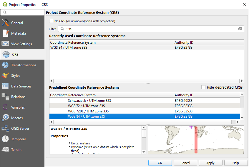
Fig. 8.3 Setting up the CRS
Save the project file by clicking on the
 Save Project toolbar button, or use the
menu item.
Save Project toolbar button, or use the
menu item.Save it in a new directory called
Rasterprac, that you should create somewhere on your computer. You will save whatever layers you create in this directory as well. Save the project asyour_name_fynbos.qgs.
8.4.4. Loading Data into the Map
In order to process the data, you will need to load the necessary layers (street names, zones, rainfall, DEM, districts) into the map canvas.
For vectors…
Click on the
 Open Data Source Manager
button in the Data Source Manager Toolbar, and enable the
Open Data Source Manager
button in the Data Source Manager Toolbar, and enable the
 Vector tab in the dialog that appears, or
use the
menu item
Vector tab in the dialog that appears, or
use the
menu itemEnsure that
 File is selected
Click on the … button to browse for vector dataset(s)
In the dialog that appears, open the
exercise_data/more_analysis/StreetsdirectorySelect the file
Street_Names_UTM33S.shpClick Open.
The dialog closes and shows the original dialog, with the file path specified in the text field next to Vector dataset(s). This allows you to ensure that the correct file is selected. It is also possible to enter the file path in this field manually, should you wish to do so.
Click Add. The vector layer will be loaded into your map. Its color is automatically assigned. You will change it later.
Rename the layer to
StreetsRight-click on it in the Layers panel (by default, the pane along the left-hand side of the screen)
Click Rename in the dialog that appears and rename it, pressing the Enter key when done
Repeat the vector adding process, but this time select the
Generalised_Zoning_Dissolve_UTM33S.shpfile in theZoningdirectory.Rename it to
Zoning.Load also the vector layer
admin_boundaries/Western_Cape_UTM33S.shpinto your map.Rename it to
Districts.
For rasters…
Click on the
Open Data Source Manager
button and enable the  Raster tab in
the dialog that appears, or use the
menu item
Raster tab in
the dialog that appears, or use the
menu itemEnsure that
File is selectedNavigate to the appropriate file, select it, and click Open
Do this for each of the following two raster files,
DEM/SRTM.tifandrainfall/reprojected/rainfall.tifRename the SRTM raster to
DEMand the rainfall raster toRainfall(with an initial capital)
8.4.5. Changing the layer order
Click and drag layers up and down in the Layers panel to change the order they appear in on the map so that you can see as many of the layers as possible.
Now that all the data is loaded and properly visible, the analysis can begin. It is best if the clipping operation is done first. This is so that no processing power is wasted on computing values in areas that are not going to be used anyway.
8.4.6. Find the Correct Districts
Due to the aforementioned area of investigation, we need to limit our districts to the following ones:
BellvilleCapeGoodwoodKuils RiverMitchells PlainSimon TownWynberg
Right-click on the
Districtslayer in the Layers panel.In the menu that appears, select the Filter… menu item. The Query Builder dialog appears.
You will now build a query to select only the candidate districts:
In the Fields list, double-click on the
NAME_2field to make it appear in the SQL where clause text field belowClick the IN button to append it to the SQL query
Open the brackets
Click the All button below the (currently empty) Values list.
After a short delay, this will populate the Values list with the values of the selected field (
NAME_2).Double-click the value
Bellvillein the Values list to append it to the SQL query.Add a comma and double-click to add
CapedistrictRepeat the previous step for the remaining districts
Close the brackets
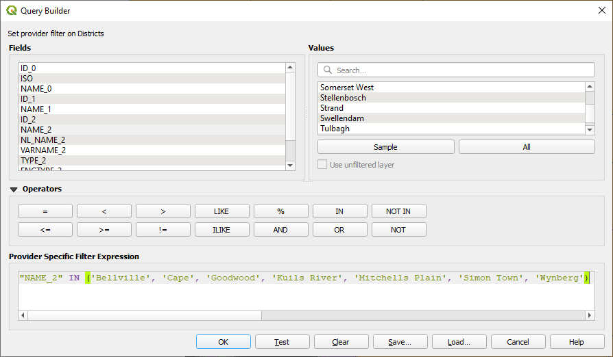
Fig. 8.4 Query builder
The final query should be (the order of the districts in the brackets does not matter):
"NAME_2" in ('Bellville', 'Cape', 'Goodwood', 'Kuils River',
             'Mitchells Plain', 'Simon Town', 'Wynberg')
Note
You can also use the
ORoperator; the query would look like this:"NAME_2" = 'Bellville' OR "NAME_2" = 'Cape' OR "NAME_2" = 'Goodwood' OR "NAME_2" = 'Kuils River' OR "NAME_2" = 'Mitchells Plain' OR "NAME_2" = 'Simon Town' OR "NAME_2" = 'Wynberg'
Click OK twice.
The districts shown in your map are now limited to those in the list above.
8.4.7. Clip the Rasters
Now that you have an area of interest, you can clip the rasters to this area.
Open the clipping dialog by selecting the menu item
In the Input layer dropdown list, select the
DEMlayerIn the Mask layer dropdown list, select the
DistrictslayerScroll down and specify an output location in the Clipped (mask) text field by clicking the … button and choosing Save to File…
Navigate to the
RasterpracdirectoryEnter a file name -
DEM_clipped.tifSave
Make sure that
 Open output file after running algorithm is checked
Click Run
After the clipping operation has completed, leave the Clip Raster by Mask Layer dialog open, to be able to reuse the clipping area
Select the
Rainfallraster layer in the Input layer dropdown list and save your output asRainfall_clipped.tifDo not change any other options. Leave everything the same and click Run.
After the second clipping operation has completed, you may close the Clip Raster by Mask Layer dialog
Save the map
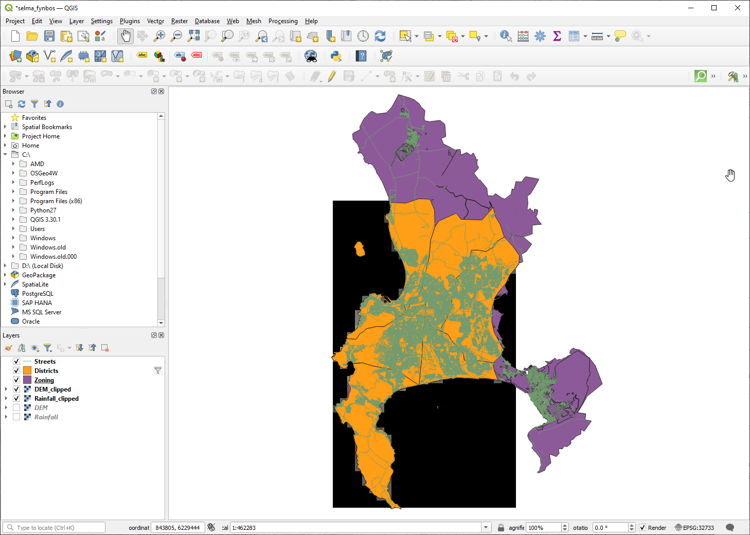
Fig. 8.5 Map view with filtered vector, clipped raster and reordered layers
Align the rasters
For our analysis we need the rasters to have the same CRS and they have to be aligned.
First we change the resolution of our rainfall data to 30 meters (pixel size):
In the Layers panel, ensure that
Rainfall_clippedis the active layer (i.e., it is highlighted by having been clicked on)Click on the menu item to open the Warp (Reproject) dialog
Under Resampling method to use, select Bilinear (2x2 kernel) from the drop down menu
Set Output file resolution in target georeferenced units to
30Scroll down to Reprojected and save the output in your
rainfall/reprojecteddirectory asRainfall30.tif.Make sure that
Open output file after running algorithm is checked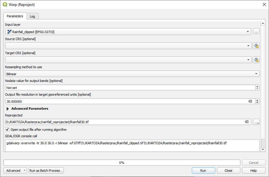
Fig. 8.6 Warp (Reproject) Rainfall_clipped
Then we align the DEM:
In the Layers panel, ensure that
DEM_clippedis the active layer (i.e., it is highlighted by having been clicked on)Click on the menu item to open the Warp (Reproject) dialog
Under Target CRS, select Project CRS: EPSG:32733 - WGS 84 / UTM zone 33S from the drop down menu
Under Resampling method to use, select Bilinear (2x2 kernel) from the drop down menu
Set Output file resolution in target georeferenced units to
30Scroll down to Georeferenced extents of output file to be created. Use the button to the right of the text box to select .
Scroll down to Reprojected and save the output in your
DEM/reprojecteddirectory asDEM30.tif.Make sure that
Open output file after running algorithm is checked
In order to properly see what’s going on, the symbology for the layers needs to be changed.
8.4.8. Changing the symbology of vector layers
In the Layers panel, right-click on the Streets layer
Select Properties from the menu that appears
Switch to the Symbology tab in the dialog that appears
Click on the Line entry in the top widget
Select a symbol in the list below or set a new one (color, transparency, …)
Click OK to close the Layer Properties dialog. This will change the rendering of the Streets layer.
Follow a similar process for the Zoning layer and choose an appropriate color for it
8.4.9. Changing the symbology of raster layers
Raster layer symbology is somewhat different.
Open the Properties dialog for the Rainfall30 raster layer
Switch to the Symbology tab. You’ll notice that this dialog is very different from the version used for vector layers.
Expand Min/Max Value Settings
Ensure that the button Mean +/- standard deviation is selected
Make sure that the value in the associated box is
2.00For Contrast enhancement, make sure it says Stretch to MinMax
For Color gradient, change it to White to Black
Click OK
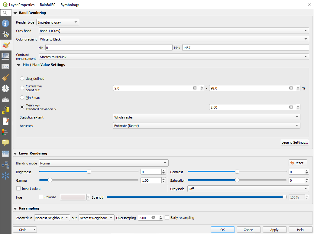
Fig. 8.7 Raster symbology
The
Rainfall30raster, if visible, should change colors, allowing you to see different brightness values for each pixelRepeat this process for the
DEM30layer, but set the standard deviations used for stretching to4.00
8.4.10. Clean up the map
Remove the original
RainfallandDEMlayers, as well asRainfall_clippedandDEM_clippedfrom the Layers panel:Right-click on these layers and select Remove.
Note
This will not remove the data from your storage device, it will merely take it out of your map.
Save the map
You can now hide the vector layers by unchecking the box next to them in the Layers panel. This will make the map render faster and will save you some time.
8.4.11. Create the hillshade
In order to create the hillshade, you will need to use an algorithm that was written for this purpose.
In the Layers panel, ensure that
DEM30is the active layer (i.e., it is highlighted by having been clicked on)Click on the menu item to open the Hillshade dialog
Scroll down to Hillshade and save the output in your
Rasterpracdirectory ashillshade.tifMake sure that
Open output file after running algorithm is checkedClick Run
Wait for it to finish processing.
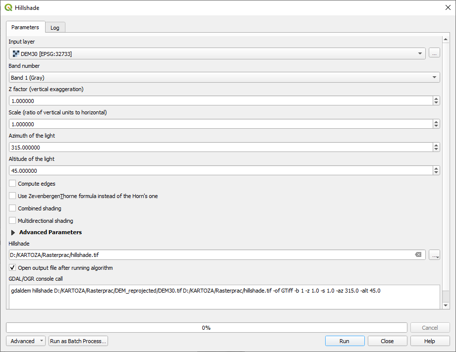
Fig. 8.8 Raster analysis Hillshade
The new hillshade layer has appeared in the
Layers panel.
Right-click on the
hillshadelayer in the Layers panel and bring up the Properties dialogClick on the Transparency tab and set the Global Opacity slider to
20%Click OK
Note the effect when the transparent hillshade is superimposed over the clipped DEM. You may have to change the order of your layers, or click off the
Rainfall30layer in order to see the effect.
8.4.12. Slope
Click on the menu item to open the Slope algorithm dialog
Select
DEM30as Input layerCheck
Slope expressed as percent instead of degrees.
Slope can be expressed in different units (percent or degrees).
Our criteria suggest that the plant of interest grows on slopes with
a gradient between 15% and 60%.
So we need to make sure our slope data is expressed as a percent.Specify an appropriate file name and location for your output.
Make sure that
Open output file after running algorithm is checkedClick Run
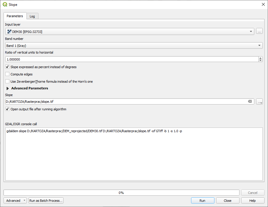
Fig. 8.9 Raster analysis Slope
The slope image has been calculated and added to the map. As usual, it is rendered in grayscale. Change the symbology to a more colorful one:
Open the layer Properties dialog (as usual, via the right-click menu of the layer)
Click on the Symbology tab
Where it says Singleband gray (in the Render type dropdown menu), change it to Singleband pseudocolor
Choose Mean +/- standard deviation x for Min / Max Value Settings with a value of
2.0Select a suitable Color ramp
Click Run
8.4.13. Try Yourself: Aspect
Use the same approach as for calculating the slope, choosing Aspect… in the menu.
Remember to save the project periodically.
8.4.14. Reclassifying rasters
Choose
Specify your
Rasterpracdirectory as the location for the Output layer (click on the … button), and save it asslope15_60.tifEnsure that the Open output file after running algorithm box is selected.
In the Raster bands list on the left, you will see all the raster layers in your Layers panel. If your Slope layer is called slope, it will be listed as
slope@1. Indicating band 1 of the slope raster.The slope needs to be between
15and60degrees.Using the list items and buttons in the interface, build the following expression:
(slope@1 > 15) AND (slope@1 < 60)
Set the Output layer field to an appropriate location and file name.
Click Run.
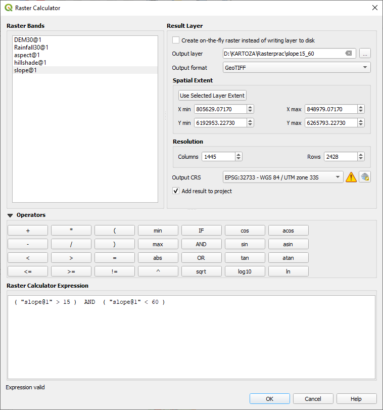
Fig. 8.10 Raster calculator Slope
Now find the correct aspect (east-facing: between 45 and 135
degrees) using the same approach.
Build the following expression:
(aspect@1 > 45) AND (aspect@1 < 135)
You will know it worked when all of the east-facing slopes are white in the resulting raster (it’s almost as if they are being lit by the morning sunlight).
Find the correct rainfall (greater than 1000 mm) the same way.
Use the following expression:
Rainfall30@1 > 1000
Now that you have all three criteria each in separate rasters, you
need to combine them to see which areas satisfy all the criteria.
To do so, the rasters will be multiplied with each other.
When this happens, all overlapping pixels with a value of 1 will
retain the value of 1 (i.e. the location meets the criteria), but
if a pixel in any of the three rasters has the value of 0 (i.e.
the location does not meet the criteria), then it will be 0 in the
result.
In this way, the result will contain only the overlapping areas that
meet all of the appropriate criteria.
8.4.15. Combining rasters
Open the Raster Calculator ()
Build the following expression (with the appropriate names for your layers):
[aspect45_135] * [slope15_60] * [rainfall_1000]
Set the output location to the
RasterpracdirectoryName the output raster
aspect_slope_rainfall.tifEnsure that
Open output file after running algorithm is checkedClick Run
The new raster now properly displays the areas where all three criteria are satisfied.
Save the project.
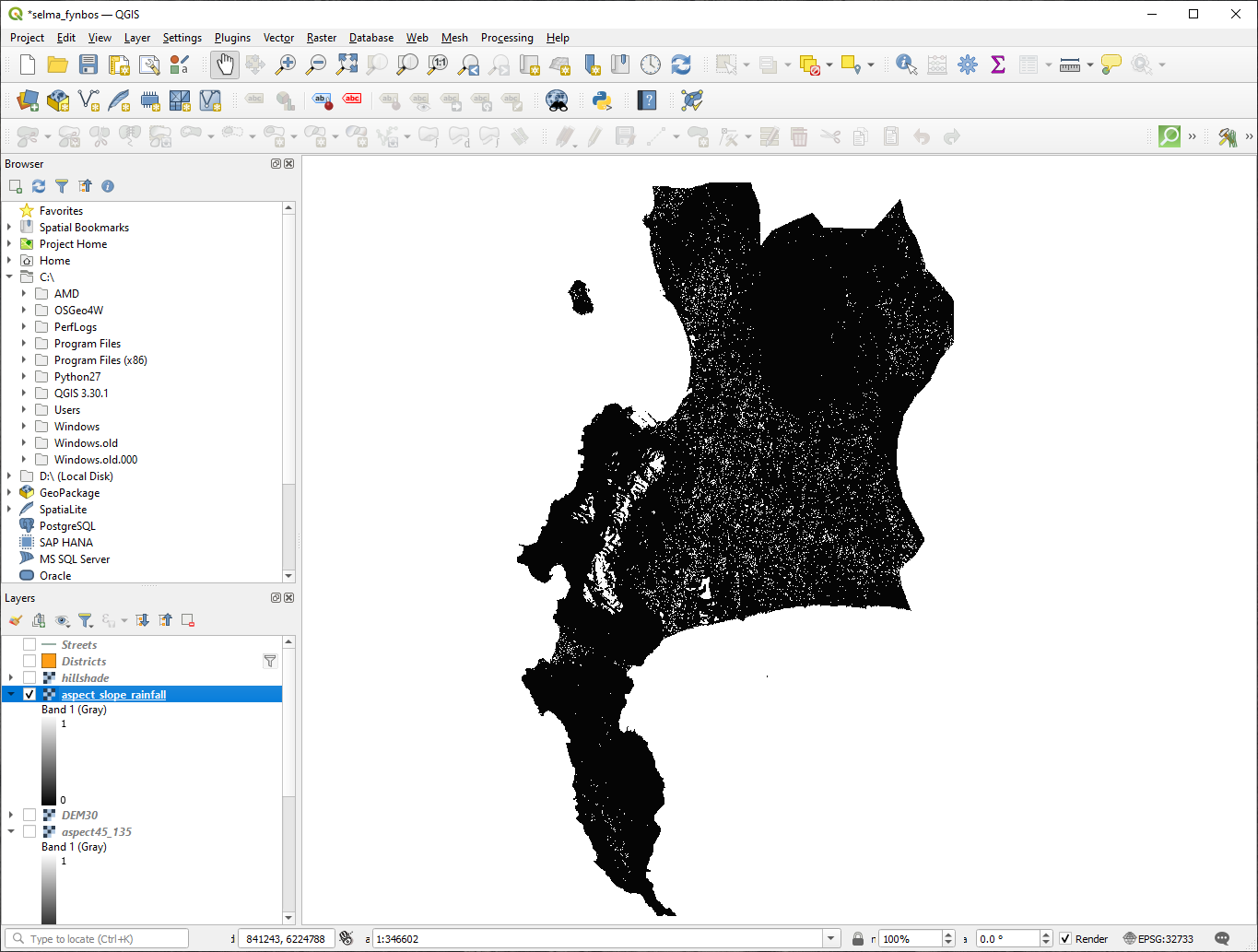
Fig. 8.11 Map view where all three criteria are satisfied
The next criterion that needs to be satisfied is that the area must be
250 m away from urban areas.
We will satisfy this requirement by ensuring that the areas we compute
are inside rural areas, and are 250 m or more from the edge of the area.
Hence, we need to find all rural areas first.
8.4.16. Finding rural areas
Hide all layers in the Layers panel
Unhide the
Zoningvector layerRight-click on it and bring up the Attribute Table dialog. Note the many different ways that the land is zoned here. We want to isolate the rural areas. Close the Attribute table.
Right-click on the
Zoninglayer and select Filter… to bring up the Query Builder dialogBuild the following query:
"Gen_Zoning" = 'Rural'
See the earlier instructions if you get stuck.
Click OK to close the Query Builder dialog. The query should return one feature.
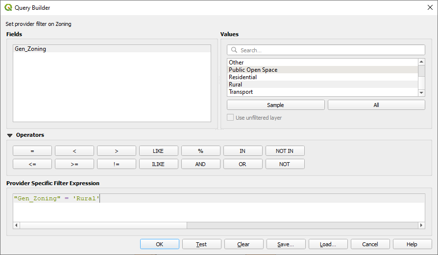
Query builder Zoning
You should see the rural polygons from the Zoning layer.
You will need to save these.
In the right-click menu for
Zoning, select .Save your layer under the
RasterpracdirectoryName the output file
rural.shpClick OK
Save the project
Now you need to exclude the areas that are within 250m from the
edge of the rural areas.
Do this by creating a negative buffer, as explained below.
8.4.17. Creating a negative buffer
Click the menu item
In the dialog that appears, select the
rurallayer as your input vector layer (Selected features only should not be checked)Set Distance to
-250. The negative value means that the buffer will be an internal buffer. Make sure that the units are meters in the dropdown menu.Check
Dissolve resultIn Buffered, place the output file in the
Rasterpracdirectory, and name itrural_buffer.shpClick Save
Click Run and wait for the processing to complete
Close the Buffer dialog.
Make sure that your buffer worked correctly by noting how the
rural_bufferlayer is different from therurallayer. You may need to change the drawing order in order to observe the difference.Remove the
rurallayerSave the project
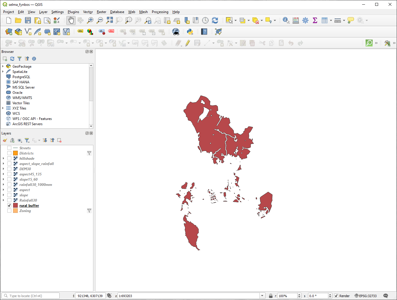
Fig. 8.12 Map view with rural buffer
Now you need to combine your rural_buffer vector layer with the
aspect_slope_rainfall raster.
To combine them, we will need to change the data format of one of the
layers. In this case, you will vectorize the raster, since vector
layers are more convenient when we want to calculate areas.
8.4.18. Vectorizing the raster
Click on the menu item
Select the
aspect_slope_rainfallraster as Input layerSet Name of the field to create to
suitable(the default field name isDN- Digital number data)Save the output. Under Vectorized, select Save file as. Set the location to
Rasterpracand name the fileaspect_slope_rainfall_all.shp.Ensure that
Open output file after running algorithm is checkedClick Run
Close the dialog when processing is complete
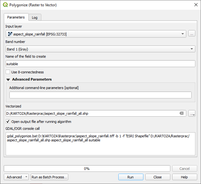
Fig. 8.13 Raster to Vector
All areas of the raster have been vectorized, so you need to select
only the areas that have a value of 1 in the suitable field.
(Digital Number.
Open the Query Builder dialog (right-click - Filter…) for the new vector layer
Build this query:
"suitable" = 1
Click OK
After you are sure the query is complete (and only the areas that meet all three criteria, i.e. with a value of
1are visible), create a new vector file from the results, using the in the layer’s right-click menuSave the file in the
RasterpracdirectoryName the file
aspect_slope_rainfall_1.shpRemove the
aspect_slope_rainfall_alllayer from your mapSave your project
When we use an algorithm to vectorize a raster, sometimes the algorithm yields what is called “Invalid geometries”, i.e. there are empty polygons, or polygons with mistakes in them, that will be difficult to analyze in the future. So, we need to use the “Fix Geometry” tool.
8.4.19. Fixing geometry
In the Processing Toolbox, search for “Fix geometries”, and Execute… it
For the Input layer, select
aspect_slope_rainfall_1Under Fixed geometries, select Save file as, and save the output to
Rasterpracand name the filefixed_aspect_slope_rainfall.shp.Ensure that
Open output file after running algorithm is checkedClick Run
Close the dialog when processing is complete
Now that you have vectorized the raster, and fixed the resulting
geometry, you can combine the aspect, slope, and rainfall criteria
with the distance from human settlement criteria by finding the
intersection of the fixed_aspect_slope_rainfall layer and the
rural_buffer layer.
8.4.20. Determining the Intersection of vectors
Click the menu item
In the dialog that appears, select the
rural_bufferlayer as Input layerFor the Overlay layer, select the
fixed_aspect_slope_rainfalllayerIn Intersection, place the output file in the
RasterpracdirectoryName the output file
rural_aspect_slope_rainfall.shpClick Save
Click Run and wait for the processing to complete
Close the Intersection dialog.
Make sure that your intersection worked correctly by noting that only the overlapping areas remain.
Save the project
The next criteria on the list is that the area must be greater than
6000 ㎡.
You will now calculate the polygon areas in order to identify the
areas that are the appropriate size for this project.
8.4.21. Calculating the area for each polygon
Open the new vector layer’s right-click menu
Select Open attribute table
Click the
 Toggle editing button in the top
left corner of the table, or press Ctrl+e
Toggle editing button in the top
left corner of the table, or press Ctrl+eClick the
 Open field calculator button in
the toolbar along the top of the table, or press Ctrl+i
Open field calculator button in
the toolbar along the top of the table, or press Ctrl+iIn the dialog that appears, make sure that
Create new field is checked, and set the
Output field name to areaThe output field type should be a decimal number (real). Set Precision to1(one decimal).In the Expression area, type:
$area
This means that the field calculator will calculate the area of each polygon in the vector layer and will then populate a new integer column (called
area) with the computed value.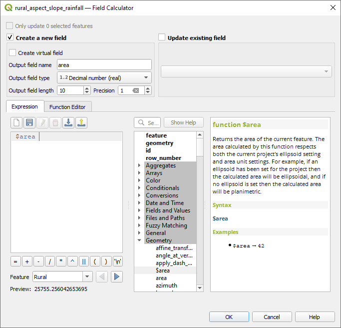
Fig. 8.14 Field Calculator
Click OK
Do the same thing for another new field called
id. In Field calculator expression, type:$id
This ensures that each polygon has a unique ID for identification purposes.
Click
Toggle editing again, and save your
edits if prompted to do so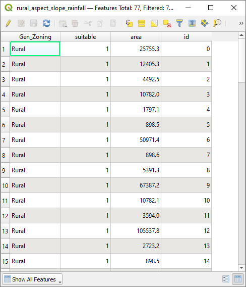
Fig. 8.15 Attribute table with area and id columns
8.4.22. Selecting areas of a given size
Now that the areas are known:
Build a query (as usual) to select only the polygons that are larger than
6000㎡. The query is:"area" > 6000
Save the selection in the
Rasterpracdirectory as a new vector layer calledsuitable_areas.shp.
You now have the suitable areas that meet all of the habitat criteria for the rare fynbos plant, from which you will pick the four areas that are nearest to the University of Cape Town.
8.4.23. Digitize the University of Cape Town
Create a new vector layer in the
Rasterpracdirectory as before, but this time, use Point as Geometry type and name ituniversity.shpEnsure that it is in the correct CRS (
Project CRS:EPSG:32733 - WGS 84 / UTM zone 33S)Finish creating the new layer (click OK)
Hide all layers except the new
universitylayer and theStreetslayer.Add a background map (OSM):
Go to the Browser panel and navigate to
Drag and drop the
OpenStreetMapentry to the bottom of the Layers panel
Using your internet browser, look up the location of the University of Cape Town. Given Cape Town’s unique topography, the university is in a very recognizable location. Before you return to QGIS, take note of where the university is located, and what is nearby.
Ensure that the
Streetslayer clicked on, and that theuniversitylayer is highlighted in the Layers panelNavigate to the menu item and ensure that Digitizing is selected. You should then see a toolbar icon with a pencil on it (
Toggle editing).
This is the Toggle Editing button.Click the Toggle editing button to enter edit mode. This allows you to edit a vector layer
Click the
 Add Point Feature button, which
should be nearby the Toggle editing button
Add Point Feature button, which
should be nearby the Toggle editing buttonWith the Add feature tool activated, left-click on your best estimate of the location of the University of Cape Town
Supply an arbitrary integer when asked for the
idClick OK
Click the
 Save Layer Edits button
Click the Toggle editing button to stop your editing session
Save the project
8.4.24. Find the locations that are closest to the University of Cape Town
Go to the Processing Toolbox, locate the Join Attributes by Nearest algorithm () and execute it
Input layer should be
university, and Input layer 2suitable_areasSet an appropriate output location and name (Joined layer)
Set the Maximum nearest neighbors to
4Ensure that
Open output file after running algorithm is checkedLeave the rest of the parameters with their default values
Click Run
The resulting point layer will contain four features - they will
all have the location of the university and its attributes, and in
addition, the attributes of the nearby suitable areas (including the
id), and the distance to that location.
Open the attribute table of the result of the join
Note the
idof the four nearest suitable areas, and then close the attribute tableOpen the attribute table of the
suitable_areaslayerBuild a query to select the four suitable areas closest to the university (selecting them using the
idfield)
This is the final answer to the research question.
For your submission, create a fully labeled layout that includes the
semi-transparent hillshade layer over an appealing raster of your
choice (such as the DEM or the slope raster,
for example).
Also include the university and the suitable_areas layer, with
the four suitable areas that are closest to the university
highlighted.
Follow all the best practices for cartography in creating your output
map.